Discrimination and Constraints: Evidence from The Voice

Table of Links

Abstract

Background

Data

Methodology

Results

Discussion and Conclusion, and References

A Appendix Tables and Figures

4 Results

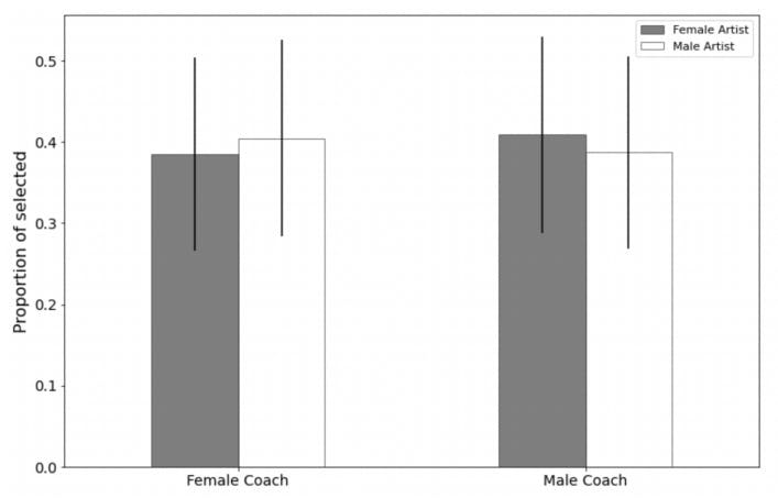
My identification strategy is to leverage the exogenous assignment of coaches to the artist and use a difference-in-differences estimator across these coach-artist interactions to estimate the degree of gender bias in selection. The baseline difference in differences results shows that female coaches are more likely to choose male artists, and male coaches are more likely to select female artists, opposite gender bias (Figure 1). A simple calculation suggests an opposite gender bias of 4.2 percentage points.

Notes: This figure reports the share of selected male and female artists assigned to male and female coaches. There is a statistical difference in the selection of female artists assigned to female or male coaches. The same is true for male artists.

4.1 Effect of Own-Gender Coaches on Selection

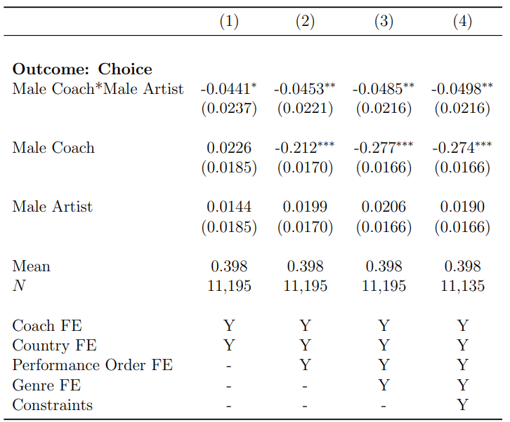
Table 3 reports results from estimating Equation 1 using four separate specifications. The ”same gender coach” difference in differences coefficient shows how much more or less likely an artist is to be chosen by a coach of a different gender relative to one of the same genders as the artist, adjusted for overall gender propensities of artists to get selected and coaches to choose. According to Table 3, the results represent the regression outcome of the chosen dependent variable artist. Overall, it can be seen that the primary independent variable interaction between the gender of the coach and artist is showing consistent output with controlling various confounders. The outcome gives ranges of - 4.4 and - 5 percentage points, indicating that magnitude increases with covariates. Standard errors also decreased and showed a range of 15% and 9% for the margin of error or alpha level.

Column (1) of Table 3, includes coach and country effects and no other controls. The estimated degree of gender bias for selection in the male/female comparison is -4.4 percentage points. That is, after adjusting for gender-specific differences in propensities for contestants to perform and adjusting for gender-specific differences in coaches’ propensities to select, a male contestant who is exogenously assigned a male coach is 4.4 percentage points less likely to be chosen relative to a male contestant who is exogenously assigned a female coach (and vice versa). Given a mean of 39.75 percent, the pooled result indicates that gender bias causes a contestant assigned an other-gender coach to be nearly 11 percent more likely to be selected for any performance.

Notes: Table 3 presents a difference in differences estimate of gender bias using regression of Equation 1. This table reports the coefficient on the interaction of Male Artist and Male Coach from the regression of Choice on indicators for coach gender, artist gender, and the interaction term. Each specification includes coach and country fixed effects. Column 2 adds the order of the performance fixed effects. Column 3 includes the same controls as column 3, with the exception of adding genre-fixed effects. Column 4 adds controls for the number of males relative to females in the team, the failure rate of the coach for female artists, and the failure rate of the coach for male artists. Standard errors are clustered by coach. * p < 0.1, ** p < 0.05, *** p < 0.01

The additional columns of Table 3, address potential confounders to this gender bias estimate. Column (2) adds the order of the performance fixed effect to the coach fixed effect to account for order trends; results in these columns slightly increase in magnitude compared with those in Column (1). I have also included genre covariates in Column (3), which means coaches of a particular gender disproportionately favor certain genre styles. Suppose contestants of a different gender from these coaches are disproportionately likely to choose genre style. In that case, failure to control for genre covariates could result in a spurious gender bias estimate. In Column (4), I have incorporated the show-related specification, which I specify as constraints to the coaches. It comes from the coaches having a limited slot in their team, which will be a confounding factor in getting selected. For example, if a coach has a majority of women on the team, it might push the coach to change the strategy of choosing the contestant. Similarly, the coach has been rejected by a particular gender disproportionally more, which might lead to reluctance in selecting the next same-gender contestant. By including these covariates as confounding factors, I can control for constraints imposed by this contested environment. Across these five columns, the female/male estimates range from 4.4 to 5 percentage points. These four estimates are statistically significant at p < 0.05.

To sum up, the primary result of this study is that there is meaningful oppositegender bias by coaches in a context in which the performance of contestants is exogenously assigned to the coaches. This finding contrasts significantly with the previous work of Carlsson and Eriksson (2019). They found that women (female recruiters or firms with a high share of female employees) favor women in the recruitment process. However, they did not see much evidence that men (male recruiters or firms with a high share of male employees) favor men. Results could differ due to differences in the sample studied. As the author analyzes low- and medium-skilled occupations in Sweden, there could be differences between the countries I use and Sweden. To make the comparison, I split my sample into separate countries and compared the results with Table 3. The reported coefficients for the UK, France, and Australia in Table A1 provide a similar magnitude to my initial analysis but with less precision. The standard errors are high due to the decreased sample size. Regardless, Germany has a null coefficient. Thus, there could be differences in the results due to the context of the country. Again, I account for this discrepancy in my initial analysis by controlling for country-fixed effects. The remainder of this manuscript examines heterogeneity in these effects to better characterize the nature of this gender bias and shed light on the likely mechanisms.

4.2 Effect of Own and Opposite Gender Coaches by Constraints

Given the findings discussed above, it is natural to ask whether the differences by gender are due to only a handful of coaches or if they are more systemic. To address this question, the remainder of the empirical results examines heterogeneity in the estimated gender bias by confounding factors - team gender composition, order of performance, and failure rates of the coaches. We also discuss the extent to which difference-in-difference estimates are sensitive to these confounding factors. To do so, I use the causal forest approach described in Section 4 to estimate the heterogeneous effects of gender bias.

Because the difference in differences estimator can only identify relative gender bias across coaches, it does not show gender bias separately for male and female coaches. There could be a case when the likelihood of male coaches preferring female artists is more than female coaches to female artists. If we decompose this into separate female and male coaches, male coaches prefer female artists more than male artists, and female coaches prefer female artists more than male artists. In this case, difference-in-differences estimation shows an opposite gender bias, but opposite gender bias occurs for male coaches and own-gender bias for female coaches. To observe the source of the bias, I estimate gender bias separately for men and women for a more straightforward interpretation.

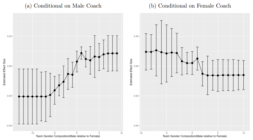
To examine heterogeneity at the coach level, I fixed coach characteristics such as coach gender. Firstly, I evaluate heterogeneity in gender bias by the gender composition of the team. To do so, I take the difference between the number of men and women in the team when the coaches hear the performance. The results of this exercise are shown in Figure 2, where the estimated effect translates into the percentage point of selecting a male artist. We can see specific local average treatment effect coefficients for gender bias when we vary team gender composition. If the majority gender group in the team is women, male coaches tend to select more female artists.

In contrast, when a majority of the team is men, male coaches tend to choose male artists, unlike female coaches, who have the opposite tendency to select opposite gender artists when a particular gender is in the minority. The exciting aspect of this analysis is that the estimated effect on the likelihood of choosing male artists is essentially centered to zero when the number of men and women in the team is equal.

I have also done the same heterogeneity analysis of gender team composition by standard ordinary least squares by grouping my dataset into males relative to the female difference in each coach’s team during the audition. According to Table A2, the estimate shows a statistically significant result when the teams are female-dominant, and the magnitude is around 8.5 percentage points of the opposite gender bias. The weight for this estimate comes from the male coach being more likely to select female artists. The analysis provides a consistent result with a causal forest estimation but has little statistical power because of the data subsets by certain cutoffs.

Notes: This figure summarizes the results from the causal forest by approach in Athey and Wager (2019), where each estimate shown represents the effect of own-gender and oppositegender interactions on selecting the artists in the case controlling for the gender of the coach and coach fixed effects. From left to right, the outcome of interest is a set of indicators for the differences in the number of male artists to the number of female artists in the team during the audition. This result effectively yields the estimates of own and opposite gender bias in selections that are specific to each team’s gender composition. Standard errors clustered by coach.

This exercise yields additional compelling evidence that gender bias, I estimate, is a systematic effect not attributable to just a handful of coaches or types of situations. Similarly, I ask whether estimates are driven by failure rates of coaches for male and female artists and the order of the artists’ performance. It is thus unsurprising to see in Figures A1, A2, and A3 that other variable-specific estimates of gender bias are uncorrelated with the failure rate of coaches for male and female artists and the order of the performance.